Phase 2 · Algorithm 10 / 30
XGBoost
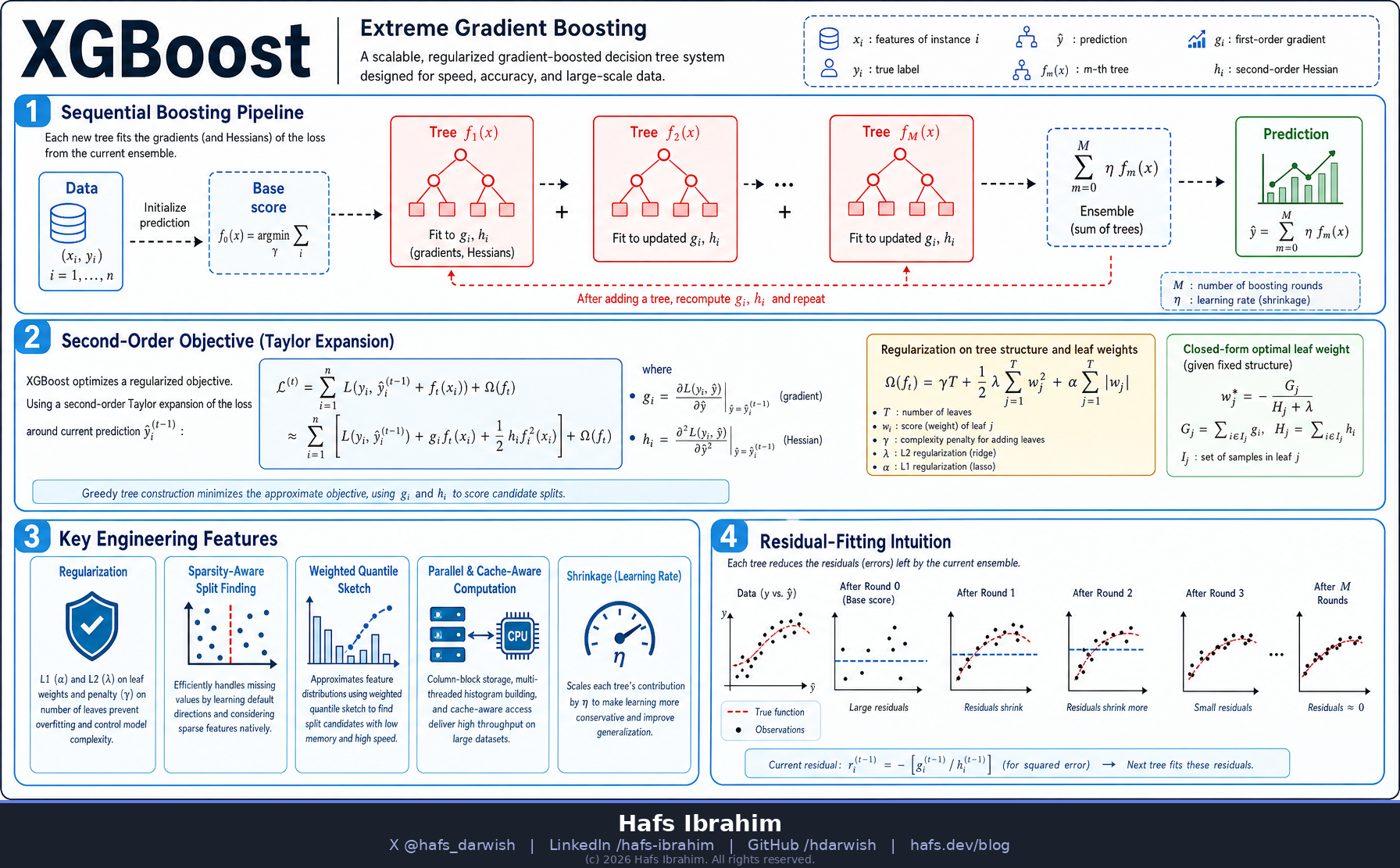
Extreme Gradient Boosting — regularized, scalable tree ensembles
Core Concept
XGBoost builds an ensemble of shallow decision trees sequentially. Each new tree is trained to correct the errors of the trees before it — but instead of just chasing residuals, it uses a second-order Taylor approximation of the loss (gradients and Hessians) and adds explicit regularization to keep trees simple. That blend of math rigor and systems engineering is why it dominated tabular ML competitions for years.
Key Components
Additive Trees
Prediction = sum of many shallow trees, added one at a time (boosting rounds).2nd-Order Objective
Uses gradient g and Hessian h of the loss — faster, more precise splits than 1st-order.Regularization Ω(f)
L1/L2 penalties on leaf weights + tree complexity fight overfitting.Systems Speed
Sparsity-aware splits, weighted quantile sketch, cache-aware parallelism.How It Works
- Start with a base prediction (e.g. the mean of the target).
- Compute the gradient g and Hessian h of the loss for every sample at the current prediction.
- Grow a new tree whose leaf weights are chosen to minimize the 2nd-order objective + Ω(f) penalty.
- Add the tree's output scaled by a learning rate η (shrinkage), then repeat for the next round.
Obj = Σ [ gᵢ·fₜ(xᵢ) + ½ hᵢ·fₜ(xᵢ)² ] + Ω(fₜ)
g = 1st-order gradient · h = 2nd-order Hessian · Ω = γT + ½λ‖w‖² regularization
Real-World Applications
Credit risk scoring
Click-through prediction
Fraud detection
Ranking / search
Kaggle tabular wins
Sales forecasting
Checkpoint Questions
- 1. Why does XGBoost use the second-order (Hessian) term when standard gradient boosting uses only the gradient? What does it buy you?
- 2. What role does the regularization term Ω(f) play, and how does it differ from the learning rate η in controlling overfitting?
- 3. "Sparsity-aware split finding" lets XGBoost handle missing values natively. How does it decide which direction a missing value should go at a split?