Variational Autoencoders
The autoencoder that learns a distribution instead of a point — so the space between examples becomes generative.
🎯Core Concept
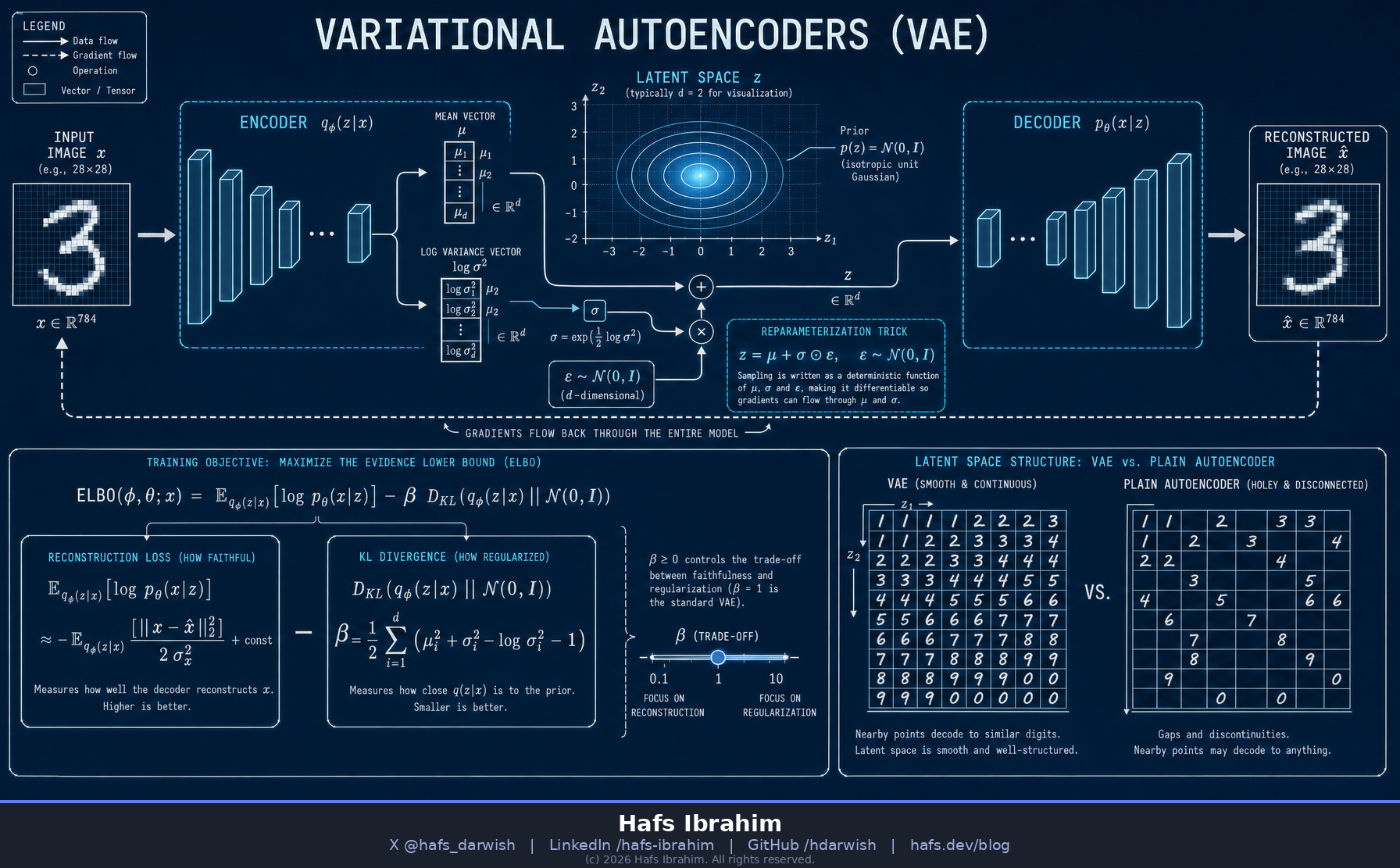
A plain autoencoder maps each input to a single point in latent space. Nothing forces those points to be arranged sensibly, so the gaps between them decode to garbage — the space is compressive but not generative.
A VAE changes the output of the encoder. Instead of one code, it emits the parameters of a distribution: a mean vector μ and a variance (usually as log σ²). You then sample a latent vector from that Gaussian and decode the sample. Because the same input maps to a small cloud rather than a dot, the decoder is forced to make every point in the neighbourhood decode to something plausible.
A second force does the rest: a KL penalty pulls all those little clouds toward a shared standard normal prior. The clouds overlap into one continuous, gap-free region. Now you can sample 𝑧 ~ N(0, I), decode, and get a new, never-seen example — that is the generative part.
🔑Key Components
Probabilistic Encoder
qφ(z|x) outputs two vectors, μ(x) and log σ²(x), not a code. Predicting the log variance keeps it unconstrained and numerically stable, since exp() guarantees positivity.
Reparameterization Trick
z = μ + σ ⊙ ε, with ε ~ N(0, I). Randomness is pushed into an input ε, so the path from loss to μ and σ is deterministic and backprop works. Sampling directly from q would block gradients.
ELBO: Two Competing Terms
Reconstruction loss says “be faithful to this input.” KL divergence says “stay close to the prior.” Training is the negotiation between fidelity and a well-shaped latent space.
The β Dial
β-VAE weights the KL term. Raise β and you get a smoother, more disentangled latent space but blurrier outputs. Lower it and you drift back toward a plain autoencoder that cannot generate.
⚙️How It Works
- Encode to a distribution. Push x through the encoder; read off μ and log σ² — a small Gaussian cloud in latent space rather than a single coordinate.
- Sample, differentiably. Draw ε ~ N(0, I) and compute z = μ + σ⊙ε. The noise enters as data, so gradients still flow to μ and σ.
- Decode and score fidelity. The decoder maps z to x̂. Reconstruction error is MSE for continuous data, Bernoulli cross-entropy for binary/pixel data.
- Regularize with KL. For a diagonal Gaussian it has a closed form: ½Σ(μ² + σ² − log σ² − 1). Zero only when μ=0 and σ=1 — the prior.
- Backprop the sum. Both terms update encoder and decoder together. The tension is the whole mechanism: fidelity alone collapses σ to zero, KL alone destroys information.
- Generate. At inference, throw the encoder away. Sample z ~ N(0, I), decode, and get a new sample. Interpolating between two z values yields a smooth morph, not noise.
📐VAE vs. Plain Autoencoder
🌎Real-World Applications
🧪Checkpoint Questions
Why can’t you just sample z directly from qφ(z|x) and train with backprop — what specifically breaks, and how does the reparameterization trick repair it?
Hint: ask where the randomness lives. Is a sampling operation a differentiable function of μ and σ, or is it a discontinuous jump? Where must ε sit for the chain rule to survive?
Suppose you train a VAE with the KL term deleted (β = 0). It reconstructs beautifully. Why does sampling z ~ N(0, I) and decoding still produce garbage?
Hint: with no pull toward the prior, where do the encoder’s clouds end up, and how wide do they get? What does the decoder then know about the region you’re sampling from?
VAE samples are famously blurrier than GAN samples. Trace that blur back to a specific term in the objective — and say when you’d still choose a VAE over a GAN anyway.
Hint: think about what minimising an expected pixel-wise reconstruction loss does when several plausible outputs exist. Then weigh it against training stability, a usable encoder, and explicit likelihood bounds.
🌳Practice Path
- Build it small. A 2-dimensional-latent VAE on MNIST, then scatter the test set’s μ values coloured by digit. You should see overlapping clouds, not islands.
- Walk the grid. Decode a uniform grid over that 2D latent plane into one image sheet. Watch digits morph continuously — that grid is the KL term made visible.
- Break it on purpose. Retrain with β = 0, then β = 5. Compare reconstruction sharpness against latent-grid smoothness. Name the tradeoff in your own words.
- Bridge forward. Read one page on latent diffusion and locate exactly where the VAE sits in the pipeline. Tomorrow’s algorithm, GANs, attacks the same problem from the opposite direction.