Algorithm 32 · Phase 8 · Generative
Generative Adversarial Networks
Two networks locked in a contest — and the contest itself is the training signal.
🧠 Mental Model
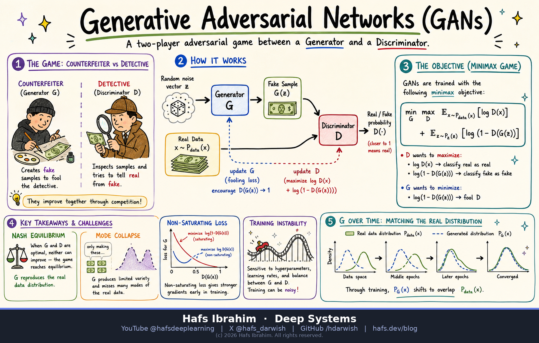
The counterfeiter and the detective. A forger prints fake notes; an inspector learns to spot them. Every time the inspector improves, the forger must improve too. Neither is given a rulebook for "what real looks like" — they extract it from each other. When the inspector can do no better than a coin flip, the forgeries are indistinguishable from reality.
🎯Core Concept
Most generative models ask you to write down a likelihood and maximise it. GANs refuse. Instead they train a Generator G that maps random noise z to samples, and a Discriminator D that scores samples as real or fake. G is never told what real data looks like — it only receives gradients passed back through D. The loss function is learned, not designed.
Formally it is a two-player minimax game with value function V:
minG maxD V(D,G) = Ex~pdata[log D(x)] + Ez~pz[log(1 − D(G(z)))]
D climbs the objective (get better at detection); G descends it (get better at fooling). At the theoretical optimum, D(x) = 0.5 everywhere and the generated distribution equals the data distribution — the game minimises the Jensen–Shannon divergence between them.
🔑Key Components
Generator G(z)
Maps a low-dimensional noise vector to data space. Learns an implicit distribution — you can sample from it but never evaluate its density. Typically transposed convolutions or an upsampling stack.
Discriminator D(x)
A binary classifier that doubles as a learned loss function. Its gradient tells G which direction in pixel/feature space looks more real. Too strong and it saturates; too weak and G gets no useful signal.
Non-Saturating Loss
Early on, D rejects fakes confidently and log(1−D(G(z))) flattens — no gradient. Fix: train G to maximise log D(G(z)) instead. Same fixed point, far healthier gradients.
Nash Equilibrium
The target is not a minimum but a saddle point where neither player can unilaterally improve. This is why GAN training oscillates rather than monotonically decreasing — the loss curve is not a progress bar.
⚙️How It Works
- Sample a batch. Draw real examples x from the dataset and noise vectors z from a simple prior (usually Gaussian or uniform).
- Generate fakes. Push z through G to get G(z) — a batch of synthetic samples.
- Update D. Take one (or k) gradient steps to maximise log D(x) + log(1 − D(G(z))). G is frozen; only the detector learns.
- Update G. Freeze D, sample fresh noise, and step G to maximise log D(G(z)). Gradients flow through D into G — D is the teacher, not the target.
- Alternate to equilibrium. Repeat. Judge progress by sample quality and metrics like FID, never by the raw loss values.
The two classic failure modes. Mode collapse — G finds one output that reliably fools D and emits only that, abandoning the diversity of the data. Training instability — the two losses chase each other in circles and never settle. Mitigations: Wasserstein loss with gradient penalty (WGAN-GP), spectral normalisation, one-sided label smoothing, and minibatch discrimination.
🌎Real-World Applications
Photorealistic synthesis — StyleGAN-class models for faces, textures, and product imagery with controllable latent directions.
Image-to-image translation — CycleGAN and pix2pix for sketch→photo, satellite→map, and style transfer without paired data.
Super-resolution — SRGAN recovers plausible high-frequency detail that pixel-wise MSE losses blur away.
Data augmentation — synthesising rare medical or defect samples to balance sharply skewed training sets.
Anomaly detection — if G cannot reconstruct a sample from its latent space, that sample is likely out-of-distribution.
Privacy-preserving data — releasing synthetic tabular records that keep statistical structure without exposing real individuals.
🧪Checkpoint Questions
Question 1
A VAE and a GAN both turn noise into samples. Why do GAN outputs tend to look sharper while VAE outputs look blurry?
Hint: ask what each model is actually being penalised for. One optimises a pixel-wise reconstruction likelihood and must hedge across all plausible outputs; the other optimises an adversary's judgement, which rewards committing to one crisp answer.
Question 2
Your discriminator reaches 99% accuracy within the first few hundred steps and the generator stops improving. Why is a too-good discriminator a problem, and what does the non-saturating loss change?
Hint: differentiate log(1−D(G(z))) when D(G(z)) is near zero. Think about gradient magnitude, not correctness.
Question 3
Both losses have plateaued and look stable. Why is that not evidence that training succeeded, and how would you actually verify it?
Hint: the objective is a saddle point in a game, not a minimum of a fixed function — the losses are relative to a moving opponent. Consider mode collapse, and what a diversity-aware metric like FID measures that the loss cannot.
🔥 Streak 33
Phase 8 · 2/10
Next: Attention Mechanisms