Diffusion Models
Learn to destroy an image, and you learn to create one.
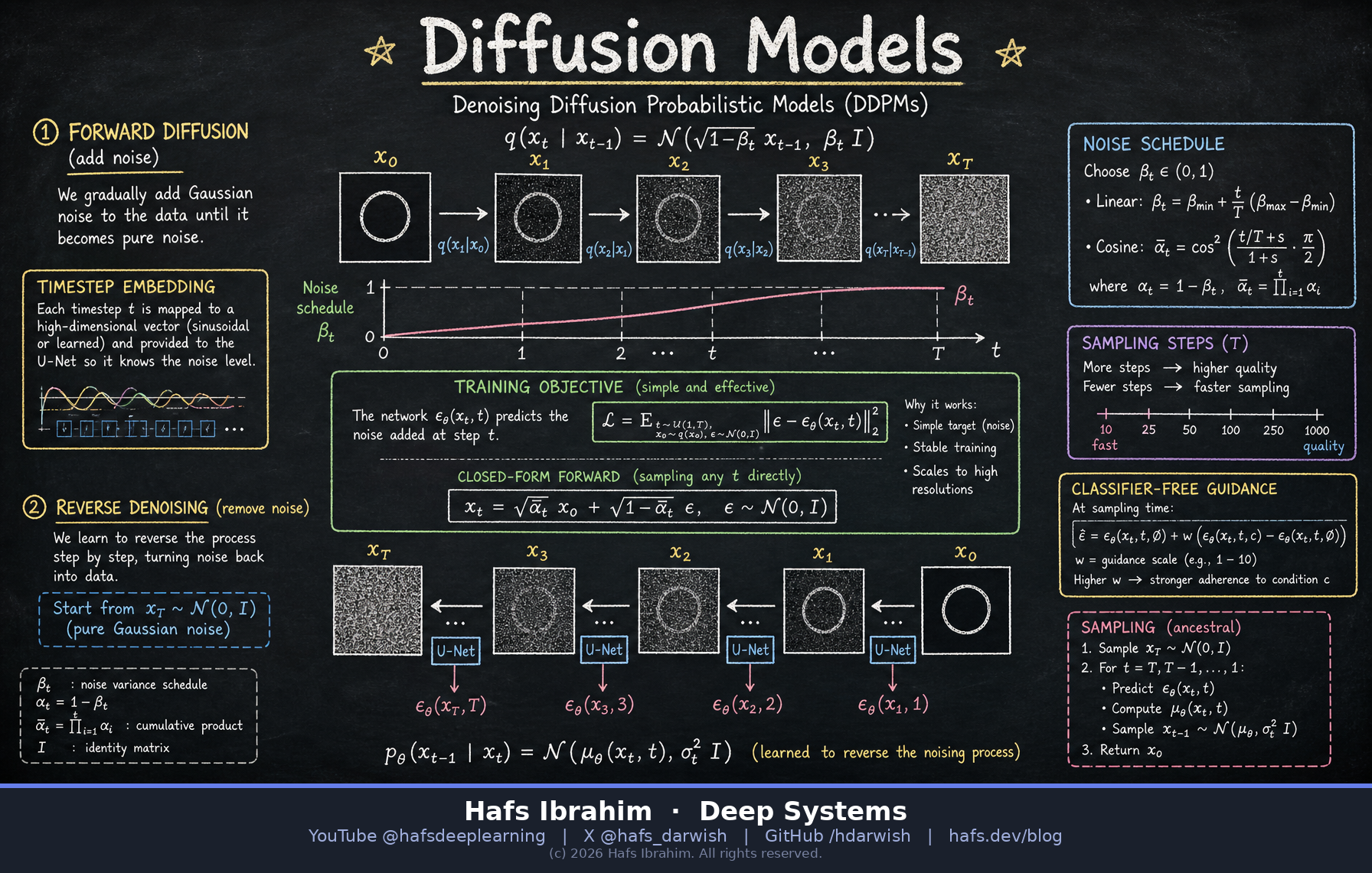
🎯 Core Concept
A diffusion model learns generation by learning destruction in reverse. Take a real image and add a little Gaussian noise, again and again, over T steps — eventually it is pure static. That forward path is fixed and needs no learning. Then train one network to answer a single, humble question at every step: “what noise was just added?” If it can answer that, you can start from pure static and walk backwards, subtracting predicted noise step by step, until a brand-new image appears that was never in your data.
🔑 Key Components
1. Forward process (fixed)
Add noise on a schedule β1..T. No parameters, no training. A closed form jumps straight to any step t, so training samples timesteps at random instead of simulating the whole chain.
2. Noise predictor εθ
A U-Net (or DiT) takes the noisy image plus a timestep embedding and predicts the noise inside it. One network handles every noise level — the timestep tells it how much fog to expect.
3. Simple loss
Plain mean-squared error between true and predicted noise. A variational bound collapses to this — which is why diffusion trains stably where GANs fight themselves.
4. Sampler + guidance
DDPM (many steps, high fidelity) vs DDIM/flow samplers (10–50 steps). Classifier-free guidance scales the gap between conditioned and unconditioned predictions to sharpen prompt adherence.
⚙️ How It Works
- Sample a real image x0 and a random timestep t in [1, T].
- Corrupt it in one shot using the closed form: xt = √ᾱt x0 + √(1-ᾱt) ε, keeping the ε you drew.
- Predict that ε from xt and t; take a gradient step on the squared error. Nothing adversarial, nothing to balance.
- To generate: start from xT ∼ N(0, I) and iterate the reverse step — subtract the predicted noise, add back a little fresh noise, repeat.
- Steer it: condition on text (cross-attention) and amplify with guidance. In latent diffusion, run all of this inside a compressed VAE space, not raw pixels — that is what made it cheap enough to ship.
🌎 Real-World Applications
🧪 Checkpoint Questions
1. Why is diffusion training so much more stable than GAN training, even though both produce images?
Hint: count the networks and the objectives. One is a regression against a target you already know; the other is a moving-target minimax game.2. The network predicts the noise ε rather than the clean image x0 directly. Both are recoverable from each other — so why does predicting noise work better?
Hint: think about what the target looks like at high t. Which parameterisation keeps the target's scale roughly constant across all timesteps?3. Cutting from 1000 sampling steps to 20 makes generation 50× faster. What are you actually trading away, and why can DDIM get away with it?
Hint: each reverse step assumes the change is small enough to be near-Gaussian. Removing the injected noise makes the trajectory deterministic — fewer, larger, straighter strides.
Card 36 of 40 · Phase 8: Modern Architectures · Visual style: chalkboard
Next up: Graph Neural Networks — learning on data that has no grid at all.