Bayesian Optimization
◆Core Concept
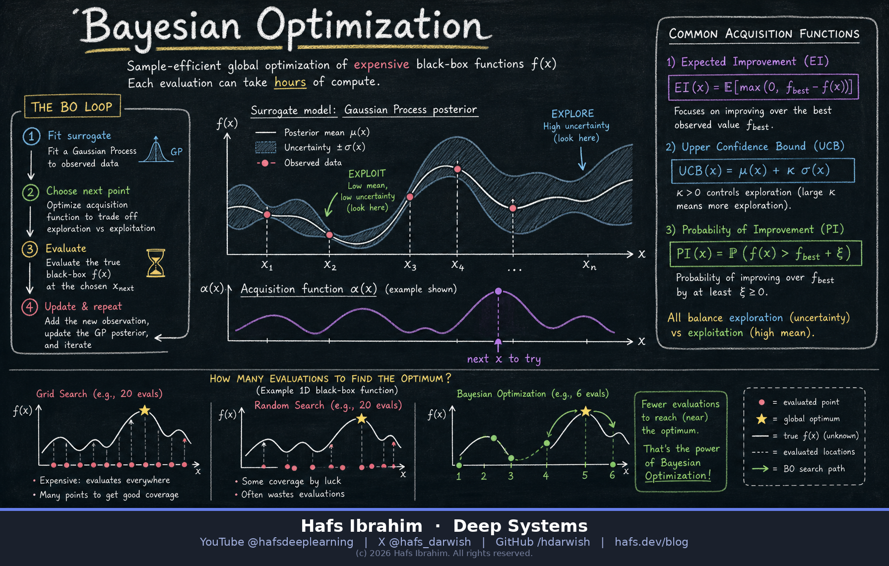
Grid search asks every question. Random search asks arbitrary questions. Bayesian Optimization asks the most informative next question — and typically finds a good optimum in tens of evaluations where random search needs thousands.
▣Key Components
1 · Surrogate Model
Usually a Gaussian Process. Gives a posterior mean μ(x) — the best guess — plus a standard deviation σ(x) that widens where you haven't looked. The uncertainty is the whole point.
2 · Acquisition Function
Turns (μ, σ) into a single "worth trying" score. Cheap to evaluate, so you can optimize it hard with gradients or random restarts. Its argmax is your next experiment.
3 · Explore / Exploit Dial
Chase low μ (exploit what looks good) or high σ (explore what's unknown). The acquisition function encodes this trade-off explicitly instead of leaving it to luck.
4 · Sequential Loop
Observe → update posterior → re-optimize acquisition → observe again. Every evaluation reshapes the belief, so the search gets smarter with each expensive step.
↻How It Works
- Seed. Evaluate f at a handful of points (Latin hypercube or Sobol, ~5–10 for low dimensions). You cannot model nothing.
- Fit the surrogate. Condition a GP on all observed pairs. Out comes μ(x) and σ(x) over the whole domain — a full posterior, not a point estimate.
- Score every candidate. Compute the acquisition function across the domain. It is analytic and cheap, so this step costs nothing compared to one real evaluation.
- Pick the argmax. The peak of the acquisition surface is your next x. Note it may sit far from the current best — that's deliberate exploration, not a bug.
- Pay for one evaluation. Run the expensive experiment at that single point. Add (x, y) to the dataset.
- Repeat until budget dies. Stop on evaluation count, wall-clock, or when expected improvement falls under a threshold. Return the best observed point.
◎Real-World Applications
- Hyperparameter tuning. Learning rate, depth, weight decay for a model that takes 8 hours per run — the canonical use case (Optuna, Ax/BoTorch, SMAC, Vizier).
- Drug & materials discovery. Each candidate compound is a physical synthesis. BO chooses which molecule to make next.
- A/B testing & pricing. Each configuration costs real traffic and revenue; BO minimizes how many bad variants users ever see.
- Robotics & control. Tuning gait or PID parameters on hardware, where each trial risks wear and a fall.
- Chip & simulation design. Layout or CFD parameters where one simulation burns hours of cluster time.
Where it breaks: GPs scale as O(n³) in observations, so past a few hundred points you switch to sparse GPs, random forests (SMAC), or TPE. It also degrades above roughly 20 dimensions unless you exploit structure — and if evaluations are cheap, plain random search is the better tool.
?Checkpoint — answer before you move on
- Why does Bayesian Optimization need a model of uncertainty — why isn't a plain regression fit of the observed points enough to choose the next point? Hint: what would a point-estimate model ever recommend outside the region you've already sampled?
- Expected Improvement and UCB both trade exploration against exploitation. What is the concrete difference in how each one lets you control that balance? Hint: count the free parameters in each formula.
- You need to tune 40 hyperparameters and each evaluation takes 2 seconds. Is Bayesian Optimization the right tool? Defend your answer with two specific reasons. Hint: think about GP cost per iteration versus the cost of one evaluation, and about dimensionality.
scikit-optimize's gp_minimize on the same function with 12 calls and compare its chosen points to yours.