Gaussian Processes
The model that answers “what’s your prediction?” and “how sure are you?” — in the same breath.
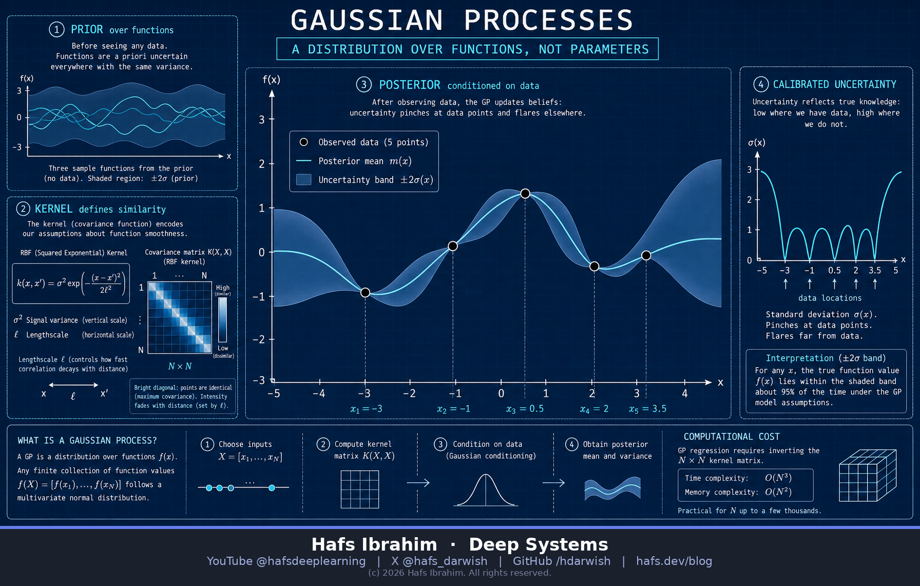
🎯 Core Concept
m(x) and a covariance given by a kernel k(x, x′). Condition that prior on your observed data and you get a posterior: a mean curve plus a calibrated error bar at every input. It is non-parametric — the data are the model — and it is exact, closed-form Bayesian inference, no sampling required.
🔑 Key Components
The Kernel (Covariance)
Encodes “how similar are two inputs?” and thereby every assumption about the function. RBF: σ²exp(−(x−x′)²/2ℓ²). The lengthscale ℓ is the wiggle rate; small ℓ means twitchy, large ℓ means smooth. Kernel choice matters more than anything else you tune.
Prior over Functions
Before data, the GP already has opinions — sample from it and you get plausible random curves, all smooth in the way the kernel dictates. This is where domain knowledge enters: periodic kernel for seasonality, linear kernel for trend, sums and products to compose them.
Posterior & Predictive Variance
Conditioning is one Gaussian identity: μ* = K*ᵗK⁻¹y, Σ* = K** − K*ᵗK⁻¹K*. Note the variance formula never touches y — uncertainty depends on where you sampled, not what you observed there.
The O(n³) Wall
Inverting an n×n matrix costs cubic time and quadratic memory. Comfortable to a few thousand points, then you need sparse/inducing-point approximations (SVGP, SoR) or structured kernels. This is the single reason GPs lost the big-data era.
⚙️ How It Works
- Choose a kernel and a mean. Usually
m(x)=0after centring; the kernel carries the real modelling decisions (smoothness, periodicity, additivity). - Build the covariance matrix
K(X,X)over yourntraining inputs, then addσₙ²Ito the diagonal for observation noise — this also keeps the matrix invertible. - Fit the hyperparameters (ℓ, signal variance, noise) by maximising the marginal likelihood. Its own built-in complexity penalty means GPs resist overfitting without a separate validation set.
- Condition on the data using the Gaussian conditioning identity — one Cholesky decomposition gives you both the posterior mean and the full covariance. No gradient descent over weights, no epochs.
- Predict with error bars. Return
μ*and±2√Σ*. Tight near data, wide in the gaps — and that widening is what downstream decision-making actually consumes.
📊 Where It Sits
| Compared to | The distinction that matters |
|---|---|
| Linear Regression | Same Bayesian machinery, but the kernel lets the function be arbitrarily flexible instead of a fixed straight line. |
| SVM (RBF) | Same kernel trick, different objective. SVM gives a margin and a hard prediction; a GP gives a full probability distribution. |
| Random Forest | RF variance is an ensemble-spread heuristic; GP variance falls out of the probability model and is properly calibrated. |
| Neural Network | NN scales to millions of points but is overconfident off-distribution. A GP is honest about ignorance — and an infinitely wide NN literally is a GP. |
| Bayesian Opt. (#40) | Yesterday’s algorithm was the consumer; today’s is the engine. The surrogate that BayesOpt optimises over is almost always a GP. |
🌎 Real-World Applications
🧪 Checkpoint Questions
Σ* = K** − K*ᵗK⁻¹K* contains no y term at all. Why is that structurally significant — and what practical capability does it unlock before you have collected any labels?
Hint: if uncertainty depends only on where you sampled and not on what you measured, you can plan an experiment or sensor layout in advance.
σₙ² was free to absorb that variation.