Card 42 / 50 Phase 9 · Probabilistic Models Style: Technical Poster

Hidden Markov Models

When you can’t see the state — only its shadow.

Hidden states, observed emissions, and the Viterbi path through the trellis

Core Concept

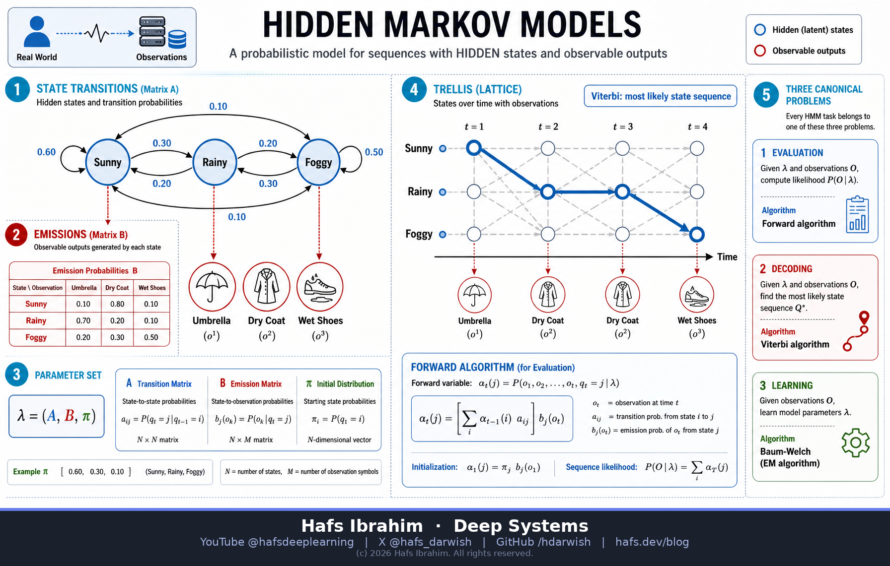
A Hidden Markov Model describes a system that moves through a sequence of hidden states you never observe directly. What you do observe are emissions — noisy signals produced by whichever state the system is in.

Two assumptions make it tractable. The Markov property: the next state depends only on the current state, not the whole history. Output independence: the current observation depends only on the current state. Everything else — forward, Viterbi, Baum-Welch — is bookkeeping over those two assumptions.

The whole model is three tables: λ = (A, B, π).

α_t(j) = [ Σ_i α_{t-1}(i) · a_ij ] · b_j(o_t)

That single recursion — sum over where you could have come from, multiply by how likely this observation is here — is the engine of the forward algorithm. Swap the sum for a max and you get Viterbi.

Key Components

A — N×N

Transition matrix

a_ij = P(state j at t+1 | state i at t). Rows sum to 1. Encodes the system’s dynamics — how sticky or jumpy the states are.

B — N×M

Emission matrix

b_j(o) = P(observation o | state j). The noisy sensor. Can be discrete counts or a continuous density (e.g. a Gaussian per state).

π — length N

Initial distribution

π_i = P(state i at t=1). Where the chain is likely to start before any evidence arrives.

Lattice

The trellis

States × time grid. Every path through it is one candidate state sequence. Dynamic programming reuses sub-paths instead of enumerating N^T of them.

The Three Canonical Problems

Evaluation

Forward algorithm — O(N²T) “How likely is this observation sequence under my model?” Accumulate α forward through the trellis. Used for scoring and model comparison.

Decoding

Viterbi — O(N²T) “What hidden sequence most likely produced this?” Same recursion with max instead of sum, plus backpointers, then trace back the single best path.

Learning

Baum-Welch (EM) — iterative “I have sequences but no labels — fit A, B, π.” E-step: forward-backward gives expected state/transition counts. M-step: re-normalise into new tables. Repeat until likelihood plateaus.

How It Works — Decoding a Sequence

Define the state space. Choose N hidden states that mean something (weather regimes, phonemes, market regimes, gene features).
Initialise the trellis. At t=1, score each state as δ₁(i) = π_i · b_i(o₁).
Recurse forward. For each later t and state j, take the best predecessor: δ_t(j) = max_i[δ_t-1(i) a_ij] · b_j(o_t), and store which i won.
Terminate. The largest δ_T(i) is the probability of the best whole path.
Backtrace. Follow the stored backpointers from T to 1 to recover the most likely hidden sequence.
Guard numerics. Probabilities multiply toward zero — work in log space (add logs) or rescale α at each step, or long sequences silently underflow.

Real-World Applications

Speech recognition. The classic use: hidden phoneme states emit acoustic feature vectors. HMM-GMM systems ran ASR for two decades before end-to-end deep models.
Part-of-speech tagging & NER. Hidden grammatical tags emit observed words; Viterbi picks the best tag sequence for a sentence.
Computational biology. Gene finding, CpG-island detection, and profile-HMMs for protein family alignment — hidden “coding / non-coding” states emit nucleotides.
Regime detection in finance. Hidden bull / bear / choppy regimes emit observed returns and volatility; useful for switching strategy parameters rather than for prediction.
Activity & sensor inference. Phone accelerometer streams → hidden walking / sitting / driving states; also gesture recognition and equipment fault-state monitoring.

Checkpoint — answer before you move on

What exactly makes the states “hidden”, and which two independence assumptions let an HMM be solved in O(N²T) instead of O(N^T)? Hint: one assumption is about the state chain, the other about the observations.
The forward algorithm and Viterbi share almost the same recursion. What is the single operator that differs, and why does that one change turn “probability of the sequence” into “best state path”? Hint: sum over all paths vs. commit to one.
Baum-Welch is EM. What does the E-step actually compute that you couldn’t just count directly, and why can Baum-Welch converge to a worse solution than a different random initialisation? Hint: expected counts from soft assignments; likelihood surface is non-convex.

Small practice: write out a 2-state HMM by hand (Sunny/Rainy, emissions Umbrella/No-Umbrella), pick simple numbers for A, B, π, and run Viterbi over three observations on paper. Doing it once by hand makes every library API obvious afterwards.