Expectation Maximization
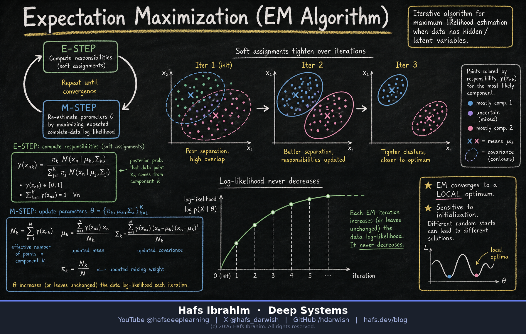
Core Concept
Maximum likelihood is easy when you can see everything. EM is what you reach for when some of the data is missing by design — the cluster label, the regime, the hidden state was never recorded.
The trick is a bargain with yourself. You cannot maximize the likelihood because it depends on unknowns, so you guess the unknowns using your current parameters (E-step), then fit parameters as if those guesses were true (M-step). Repeat. Each full turn of the loop is mathematically guaranteed never to decrease the likelihood, so the process climbs — steadily, monotonically — to a local optimum.
Read that as: average the complete-data log-likelihood over your current belief about the hidden variables, then maximize that average. Because log p(x|θ) = Q(θ|θ_old) + KL(...) with a non-negative gap, pushing Q up can never push the true likelihood down.
Key Components
Latent variable z
The thing you never observed — which Gaussian produced this point, which regime the market was in, which topic wrote this word. EM's entire reason to exist.
E-step — responsibilities
Compute the posterior γ(z_nk) = P(point n came from component k | current θ). A soft assignment: every point belongs a little to every cluster.
M-step — re-estimation
Maximize Q. For a Gaussian mixture this is a closed form: weighted means, weighted covariances, and mixing weights π_k = N_k / N.
Monotone likelihood
The convergence certificate. log p(x|θ) never decreases across an iteration, which is why you can safely stop when the change falls below a tolerance.
How It Works — Gaussian Mixture Walkthrough
- Initialize. Pick starting means, covariances, and mixing weights. In practice: run k-means first and seed EM from its centroids — it dramatically reduces bad local optima.
- E-step. For every point, compute how responsible each component is for it.
E-step: responsibility of component k for point nγ(z_nk) = π_k·N(x_n | μ_k, Σ_k) ⁄ Σ_j π_j·N(x_n | μ_j, Σ_j)
- M-step. Treat responsibilities as fractional counts and refit. With N_k = Σ_n γ(z_nk):
M-step: closed-form parameter updatesμ_k = (1/N_k) Σ_n γ(z_nk)·x_n Σ_k = (1/N_k) Σ_n γ(z_nk)(x_n−μ_k)(x_n−μ_k)ᵀ π_k = N_k / N
- Score. Evaluate log p(x|θ) = Σ_n log Σ_k π_k N(x_n|μ_k,Σ_k). It should have gone up. If it went down, you have a bug — that is EM's built-in unit test.
- Repeat until the log-likelihood change is below tolerance. Then read off the parameters, and optionally hard-assign each point to its argmax component.
The k-means connection: take a Gaussian mixture, force all covariances to σ²I and let σ² → 0. The soft responsibilities collapse to 0/1 and EM becomes exactly k-means. k-means is EM with the uncertainty deleted.
Real-World Applications
- Gaussian Mixture ModelsSoft clustering where points can straddle boundaries — customer segmentation, speaker modelling, anomaly scoring by low density.
- Baum-Welch for HMMsYesterday's algorithm. Baum-Welch is EM: forward-backward is the E-step, transition/emission re-counting is the M-step.
- Missing-data imputationSurvey and clinical data with holes. EM fills gaps with their expectation under the current model instead of a crude mean.
- Topic models & mixed-membershipDocuments as mixtures over topics; EM (and its variational cousins) recovers both topics and per-document proportions.
- Regime detection in time seriesVolatility regimes in markets — latent state is unobserved, EM estimates both regime probabilities and per-regime parameters.
Where It Bites
Local optima are real. EM guarantees you climb, not that you climb the right hill. Restart from several initializations and keep the best final likelihood.
Singular covariance collapse. A component can shrink onto a single point, driving its covariance to zero and the likelihood to infinity. Fix with a small ridge on Σ or a prior (MAP-EM).
Slow near the top. Convergence is linear, and it crawls when components overlap heavily. Fine for fitting, painful if you needed speed.
Checkpoint — answer before you move on
- Why is EM guaranteed to never decrease the observed-data log-likelihood — and why is that still not a guarantee of finding the global maximum? Hint: write log p(x|θ) as Q(θ|θ_old) plus a KL divergence, and think about what each step does to each term.
- What exactly does the E-step compute, and in what precise sense is k-means a special case of EM for a Gaussian mixture? Hint: responsibilities are a posterior. What happens to them as the shared covariance σ²I shrinks toward zero?
- A mixture component's covariance collapses toward zero during fitting and your log-likelihood explodes upward. What is happening, and what are two ways to stop it? Hint: how many data points is that component effectively explaining, and what does a prior on Σ do to the M-step?