Phase 9 · Algorithm 44 of 50

UMAP

Uniform Manifold Approximation and Projection — nonlinear dimensionality reduction that keeps the neighbourhood and the map.

Unsupervised Manifold Learning Visualization Style: sketchnote

UMAP sketchnote infographic: manifold unrolling, fuzzy k-NN graph, attractive and repulsive forces, hyperparameter knobs

Core Concept

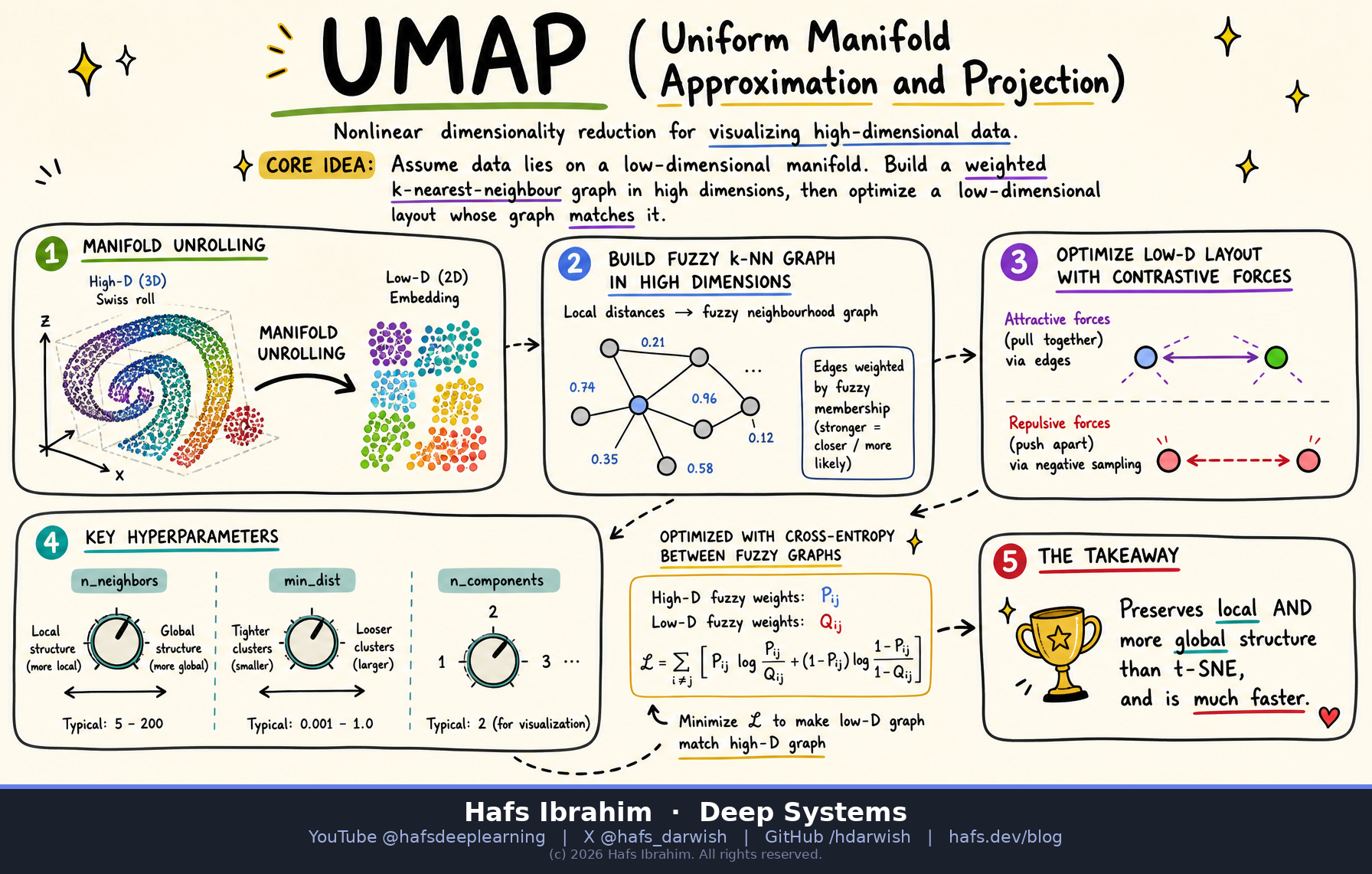
UMAP assumes your high-dimensional data actually lives on a much lower-dimensional manifold — a curved sheet folded up inside a big space. It never trusts long distances. Instead it asks each point, "who are your nearest neighbours, and how confident are you about them?", builds a fuzzy graph out of those local answers, and then lays that same graph out in 2D.

The layout is found by minimising a cross-entropy between the high-dimensional fuzzy graph and the low-dimensional one: pull connected points together, push unconnected ones apart, until the two graphs agree.

The key distinction from t-SNE: t-SNE optimises a KL divergence that only punishes putting near-neighbours far apart, so global structure drifts. UMAP's cross-entropy punishes both directions — so relative cluster placement carries more meaning, and it runs far faster on large data.

Key Components

Fuzzy k-NN Graph

Find each point's n_neighbors nearest neighbours, then convert distances to membership strengths in [0,1] using a locally adaptive kernel. Every point is guaranteed at least one edge of weight 1.

Local Connectivity Scaling

Distances are measured relative to each point's own nearest neighbour (ρ) and a bandwidth σ solved so memberships sum to log₂(k). This is what makes UMAP robust to varying density.

Low-Dim Fuzzy Model

In the embedding, edge probability is a smooth curve 1/(1 + a·d^2b), where a,b are fitted from min_dist. Small min_dist ⇒ tight, clumpy clusters.

SGD + Negative Sampling

Optimise with stochastic gradient descent: sample a real edge (attractive force), sample a few random non-edges (repulsive force). Cheap, parallel, scales to millions of points.

How It Works

Build the neighbour graph. For each point x_i, find its k nearest neighbours (approximate NN search — nearest-neighbour descent — so this is near-linear, not O(n²)).
Fuzzify local distances. Set ρ_i = distance to the closest neighbour, solve σ_i so that Σ exp(−(d(x_i,x_j) − ρ_i)/σ_i) = log₂(k). Each edge now carries a membership weight.
Symmetrise. Combine the two directed weights into one undirected weight: w = w_ij + w_ji − w_ijw_ji (a fuzzy union). You now have one weighted graph.
Initialise the embedding. Use a spectral layout (eigenvectors of the graph Laplacian) — a smart, deterministic start that already respects global shape.
Optimise by SGD. Repeatedly: pick an edge with probability ∝ its weight and pull the two points together; pick a handful of random pairs and push them apart. Learning rate decays over ~200–500 epochs.
Read the map — carefully. Cluster membership and adjacency are meaningful. Absolute distances, cluster sizes and empty-space widths are not quantitative.

Objective: C = Σ_e [ w(e)·log(w(e)/v(e)) + (1−w(e))·log((1−w(e))/(1−v(e))) ]
where w = high-dim membership, v = low-dim membership. Term 1 = attraction (don't tear neighbours apart), Term 2 = repulsion (don't falsely glue strangers together). t-SNE has only the first kind of pressure.

The Two Knobs That Matter

Parameter	Low value	High value
n_neighbors	Very local; many small fragmented clusters; fine detail	Broader view; global structure preserved; detail smoothed away
min_dist	Tight, dense clumps — good for clustering downstream	Even, spread-out points — good for seeing overall topology
metric	euclidean, cosine (text/embeddings), hamming, or a custom distance — UMAP works with any metric

Typical defaults: n_neighbors=15, min_dist=0.1, n_components=2. Always sweep n_neighbors before you believe a picture.

Real-World Applications

Single-cell genomicsThe standard tool for visualising scRNA-seq: tens of thousands of cells × 20k genes reduced to a 2D map where cell types appear as distinct islands.

Embedding inspection for LLMsProject sentence/word embeddings or hidden-layer activations to 2D to see semantic clustering, outliers, and whether your fine-tune actually separated the classes.

Preprocessing before clusteringUMAP-to-5-to-10-dims then HDBSCAN is a very strong pipeline — the reduction sharpens density contrasts the clusterer needs.

Anomaly triage and data QAPlot a labelled dataset and look for points sitting inside the wrong island — a fast visual hunt for mislabels and duplicates.

Search / recommendation debuggingMap a vector index to 2D to check whether the neighbourhoods your retriever returns actually look like coherent topic regions.

Honest caveat: UMAP is a lens, not a measurement. It is stochastic, sensitive to n_neighbors, and can manufacture visually convincing clusters from noise. Never conclude "there are 5 groups" from a UMAP plot alone — confirm with a metric on the original space.

Checkpoint — answer before you move on

Why does UMAP measure distances relative to each point's own nearest neighbour instead of using raw distances, and what would break if it didn't?Hint: think about a dataset where one region is dense and another is sparse.
UMAP minimises a cross-entropy while t-SNE minimises a KL divergence. Which extra term does UMAP's objective have, and how does that show up in the resulting picture?Hint: one of them has no pressure against putting far-apart points close together.
You increase n_neighbors from 5 to 200 and your ten crisp clusters collapse into three blobs. Which structure did you gain, which did you lose, and which setting is "correct"?Hint: neither is wrong — say what question each plot answers.

Streak: 45 days · Phase 9: Advanced & Applied · Next up: Spectral Clustering (45/50)
Try it in 10 minutes: pip install umap-learn, load sklearn.datasets.load_digits(), and plot umap.UMAP(n_neighbors=15, min_dist=0.1).fit_transform(X) coloured by digit. Then rerun with n_neighbors=3 and n_neighbors=100 and compare the three maps side by side.