Spectral Clustering
The algorithm that stops asking “how far apart are these points?” and starts asking “are these points connected?” — then lets linear algebra find the weakest place to cut.
🎯Core Concept
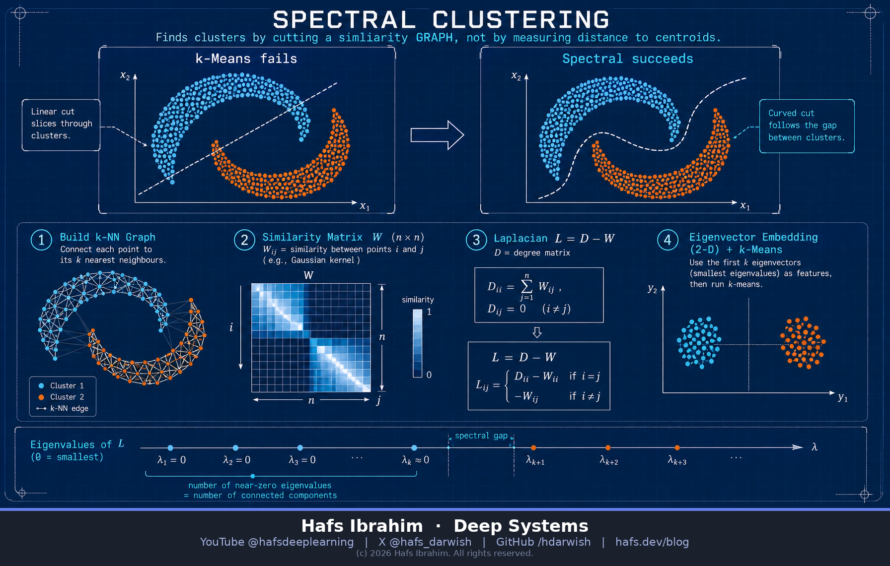
k-Means draws straight lines. That is its whole geometry — every cluster is the set of points nearest one centroid, so every boundary is a flat hyperplane. Give it two interlocking crescent moons and it slices straight through both, because the tip of one moon is genuinely closer to the other moon's belly than to its own far end.
Spectral Clustering escapes this by changing the question. It builds a graph where each point connects only to its near neighbours, and asks: where can I cut the fewest edges to split this graph in two? Along a crescent, every point has a neighbour, so the moon is one connected chain — even though its two ends are far apart. Between the moons there are almost no edges. The cheap cut is the correct cut.
The beautiful part is that you never search for that cut. You encode the graph in a matrix called the Laplacian, take its smallest eigenvectors, and those eigenvectors are a new coordinate system in which the tangled clusters have become round, well-separated blobs. Then you run plain k-means on that new space and it works trivially. Spectral clustering is not a replacement for k-means — it is a change of coordinates that makes k-means correct.
🔑Key Components
Similarity Graph (W)
Turn n points into an n×n affinity matrix. Usually a Gaussian (RBF) kernel, often sparsified to k-nearest-neighbours so far-apart points get exactly zero weight. This is where you inject your notion of “connected” — and where most of your results are decided.
Wⁱʲ = exp(−‖xⁱ − xʲ‖² / 2σ²)
Graph Laplacian (L)
Degree matrix minus weights. Its quadratic form literally measures how much a labelling disagrees across edges, so minimising it means cutting few edges. The normalised version divides out degree so dense regions don't dominate.
L = D − W · Lₖₕ = I − D⁻¹⃗² W D⁻¹⃗²
Spectral Embedding
Take the eigenvectors of the k smallest eigenvalues and stack them as columns: each point becomes a k-dimensional row. Non-convex shapes in the original space become compact, near-spherical groups here. This is the whole trick.
U = [u₁ u₂ … uₖ] → rowⁱ = embedding of xⁱ
Spectral Gap & k
The count of near-zero eigenvalues equals the number of connected components. When clusters are merely well-separated rather than disconnected, look for the largest jump between consecutive eigenvalues — that eigengap is a principled estimate of k, which k-means can never give you.
choose k = argmax (λₖ₊₁ − λₖ)
⚙️How It Works
- Build the affinity graphCompute pairwise similarity with an RBF kernel, then sparsify — keep each point's k nearest neighbours (typically 5–15) and zero the rest. You now have W.
- Form the LaplacianSum each row of W to get degrees on the diagonal of D, then L = D − W. In practice use the normalised form Lₖₕ, which is far more robust when cluster densities differ.
- Eigen-decomposeFind the k eigenvectors with the smallest eigenvalues. The first is trivially constant; the informative ones after it are the low-frequency “vibration modes” of the graph, and they bend along the natural cuts.
- Embed and row-normaliseStack those eigenvectors into an n×k matrix. In the Ng–Jordan–Weiss variant, normalise each row to unit length so points land on a sphere — this sharpens the separation.
- Cluster in the new spaceRun ordinary k-means on those k-dimensional rows. Assign each original point the label its embedded row received. Straight lines in eigenvector space are curved boundaries back in data space.
🔬Against the Neighbours
| Method | Finds non-convex shapes? | Needs k up front? | Scales to 100k+? | Handles noise? |
|---|---|---|---|---|
| k-Means | No — convex only | Yes | Yes, O(nkd) | Poor |
| DBSCAN | Yes | No | Yes, with an index | Yes — labels outliers |
| Spectral | Yes | Yes (eigengap hints) | O(n³) dense — hard | Sensitive |
| Hierarchical | Depends on linkage | No — cut later | O(n²log n) | Moderate |
- σ is the whole ballgame. Too large and the graph becomes fully connected mush; too small and it shatters into singletons. Tune it — do not accept the default and conclude spectral clustering “doesn't work”.
- O(n³) eigen-decomposition on a dense affinity matrix. Beyond ~10k points you need a sparse kNN graph plus Lanczos/ARPACK for partial eigenvectors, or Nyström approximation.
- No out-of-sample rule. A new point cannot be assigned without recomputing the embedding — unlike k-means, which just compares to centroids. Spectral clustering is transductive, not a trained model.
- A thin bridge of noise between two clusters can merge them, because the cut is no longer cheap. Denoise first.
🌎Real-World Applications
🧪Checkpoint Questions
Two interlocking crescent moons defeat k-means but not spectral clustering. Explain why in terms of what each algorithm treats as “the same cluster” — not just “spectral handles non-convex shapes”.
Hint: two points at opposite tips of one moon are far apart in Euclidean distance. What makes them nonetheless one group? Think about a chain of neighbours versus a single distance measurement to a centroid.If your graph splits into 3 truly disconnected pieces, the Laplacian has exactly 3 zero eigenvalues. Why would that fact stop being exactly true — but stay useful — when the pieces are merely weakly connected?
Hint: zero eigenvalues become small-but-nonzero ones. What does the size of the gap to the next eigenvalue tell you about how confident the split is? This is why the eigengap is a heuristic and not a theorem.You have 500,000 points and spectral clustering is the theoretically right choice. Name the specific step that breaks, and argue whether you should approximate it or switch to DBSCAN instead.
Hint: which step is cubic in n, and what property of a kNN graph could rescue it? Then weigh that against what DBSCAN gives you for free — and what it costs you when cluster densities differ.Next up: LightGBM — how histogram binning and leaf-wise growth make gradient boosting fast enough to train on millions of rows before lunch.