LightGBM
Gradient boosting rebuilt for speed: bin the features, grow the tree leaf-first, and throw away the data that no longer teaches you anything.
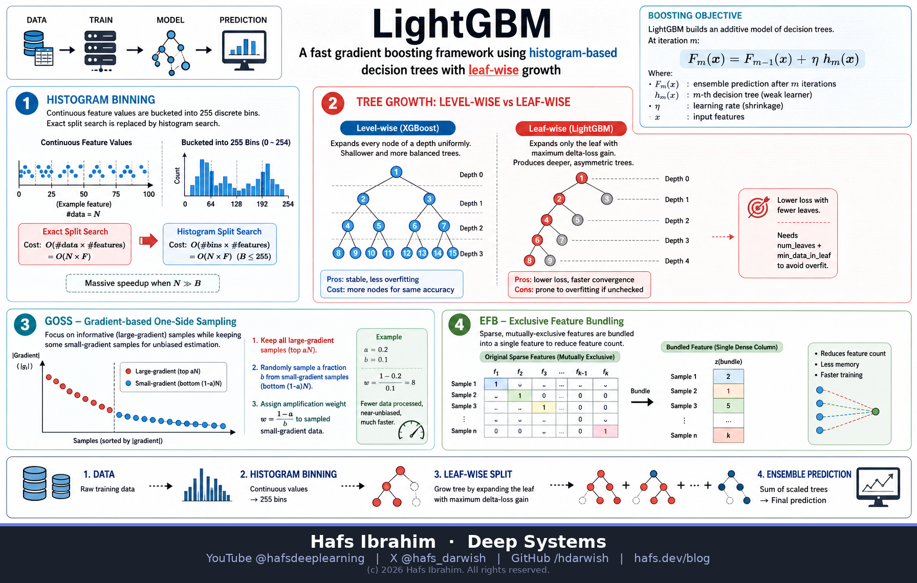
Hero generated with gpt-image-2 · style: technical-poster
Core Concept
LightGBM is gradient boosting where every expensive step has been replaced by a cheaper approximation that barely costs accuracy. Like all boosting, it fits trees sequentially, each one predicting the residual gradient of the loss so far:
Fm(x) = Fm−1(x) + η · hm(x)The innovation is not the objective — it is the engineering of the split search. Exact gradient boosting scans every distinct value of every feature at every node: O(#data × #features). LightGBM buckets each feature into ~255 histogram bins once, up front, then scans bins instead of rows: O(#bins × #features). Then it grows leaf-wise instead of level-wise, spending each new split where the loss drop is largest. Then GOSS drops most of the small-gradient (already-well-fit) rows, and EFB bundles mutually-exclusive sparse features into one. Four multiplications of speed stacked on the same math.
Key Components
Histogram Binning
Continuous features are pre-bucketed into a fixed number of bins (default 255). Split gain is computed by accumulating gradient/hessian sums per bin — one pass, tiny memory, and a child histogram can be derived by subtracting the smaller sibling from the parent.
Leaf-wise Growth
Instead of expanding a whole depth level, split the single leaf with the largest Δloss. Same number of leaves buys lower training loss — but trees get deep and asymmetric, so num_leaves and min_data_in_leaf are your real regularizers.
GOSS
Gradient-based One-Side Sampling: keep the top a% of rows by |gradient| (the badly-fit, informative ones), randomly sample b% of the rest, and up-weight those survivors by (1−a)/b so the gain estimate stays unbiased.
EFB
Exclusive Feature Bundling: in sparse data (one-hot, bag-of-words) features rarely fire together. Bundle mutually-exclusive features into one by offsetting their bin ranges — #features shrinks toward #bundles with no information lost.
How It Works
- Bin once. Before any tree is built, each feature's values are mapped to bin indices. This is a one-time O(#data × #features) pass; everything after operates on compact integers.
- Compute gradients. For the current ensemble Fm−1, compute each row's first-order gradient gi and second-order hessian hi of the loss.
- Subsample rows with GOSS. Sort by |gi|, keep all the large-gradient rows, sample the small-gradient tail, reweight it. Most of the data is skipped without skewing the split gains.
- Build histograms. For the surviving rows, accumulate Σg and Σh into each feature's bins. Use the parent-minus-sibling trick so only the smaller child is ever scanned.
- Pick the best leaf, then the best split. Across all current leaves and all bins, choose the (leaf, feature, bin) with maximum gain — that is the leaf-wise step. Grow until
num_leavesis reached. - Add the tree, shrunk. Append η·hm(x) to the ensemble and repeat. Early stopping on a validation set decides when to stop adding trees.
LightGBM vs XGBoost — the honest table
| Dimension | LightGBM | XGBoost (hist mode) |
|---|---|---|
| Tree growth | Leaf-wise (best-first) | Level-wise by default |
| Speed on wide/large data | Usually fastest; GOSS + EFB compound | Fast, but scans more rows/features |
| Small datasets | Overfits easily — cap num_leaves, raise min_data_in_leaf | More forgiving out of the box |
| Categoricals | Native optimal-split handling | Needs encoding (or newer native support) |
| Key knobs | num_leaves, min_data_in_leaf, learning_rate, feature_fraction | max_depth, eta, subsample, colsample |
Real-World Applications
- Click-through & ad rankingBillions of sparse one-hot rows — exactly the regime EFB and histogram binning were designed for. Trains in minutes where exact boosting takes hours.
- Credit risk & fraud scoringTabular, mixed categorical/numeric, class-imbalanced. LightGBM + monotonic constraints is still a production default over deep nets.
- Demand and price forecastingLag/rolling features fed to LightGBM won or placed top-10 in most recent M5-style forecasting competitions.
- Learning-to-rank search resultsBuilt-in
lambdarankobjective optimizes NDCG directly for query-grouped relevance data. - Fast baselines in any tabular ML projectTen minutes to a strong, feature-importance-explaining benchmark that your neural model must actually beat.
The Pitfall To Remember
num_leaves well below 2max_depth, set min_data_in_leaf to something real (20–100+), and let early stopping on a held-out fold decide the tree count.Checkpoint — answer before you move on
- Why does histogram binning reduce split-finding cost from O(#data × #features) to O(#bins × #features), and what accuracy do you pay for it? Hint: what exactly gets lost when 10,000 distinct values collapse into 255 buckets — and how often does the optimal split fall strictly inside a bucket?
- Leaf-wise growth reaches a lower training loss than level-wise for the same number of leaves. Explain the mechanism — and explain why that same property makes it dangerous on small datasets. Hint: think about which leaf gets the next split, and what happens when the largest remaining Δloss comes from isolating outliers.
- GOSS throws away most small-gradient rows yet claims an unbiased gain estimate. What is the reweighting factor, and why is it (1−a)/b rather than 1? Hint: the sampled tail must stand in for the whole tail. What scaling makes its summed gradient contribution match the population it represents?