Algorithm 49 / 50 Phase 9 · Advanced RL Style: Blueprint

Proximal Policy Optimization Improve the policy as much as you can — but never trust one update too far.

Blueprint-style schematic of Proximal Policy Optimization: clipped surrogate objective, rollout loop, and GAE advantage estimation

Core Concept

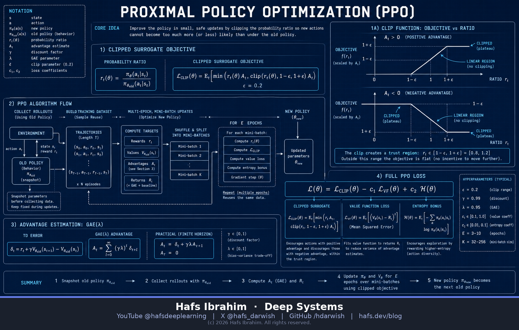
Vanilla policy gradient has one fatal habit: a single large step can destroy a working policy, and there is no way back — the data that would correct it was collected by the policy you just wrecked. PPO fixes this with a deliberately pessimistic objective.

It measures how far the new policy has moved from the one that gathered the data using the probability ratio, then refuses to reward movement beyond a small band around 1.0. Inside the band you get the full policy-gradient signal. Outside it, the gradient goes flat — the objective simply stops paying for further drift.

r_t(θ) = π_θ(a_t|s_t) / π_{θ_old}(a_t|s_t) L^CLIP = Ê_t[ min( r_tÂ_t , clip(r_t, 1−ε, 1+ε) · Â_t ) ] ε ≈ 0.2. The min is what makes it a lower bound: it always takes the less optimistic of the raw and the clipped term, so the update can never be talked into a big step by a big advantage.

That is the whole trick. TRPO achieved the same trust-region guarantee with a KL constraint and second-order optimisation. PPO throws that machinery away and gets comparable performance with first-order SGD and about twenty lines of code — which is why it became the default.

Key Components

Probability Ratio

How much more (or less) likely the current policy makes the action the old policy took. 1.0 means no change. This replaces logπ as the thing you differentiate, and it is what makes off-policy sample reuse legitimate.

r = πθ / πθ_old

Clipped Surrogate

The pessimism engine. Clamps the ratio to [1−ε, 1+ε] and takes the minimum against the unclipped term, producing a flat plateau where further drift earns nothing. No plateau, no trust region.

min(rA, clip(r)A)

GAE Advantage

Generalized Advantage Estimation: an exponentially-weighted average of n-step TD errors. λ dials the bias–variance trade-off — λ=0 is low-variance TD, λ=1 is unbiased Monte Carlo.

Â = Σ(γλ)^lδ_t+l

Composite Loss

Policy term, a value-function regression term to train the critic that produced those advantages, and an entropy bonus that keeps the policy from collapsing to determinism before it has finished exploring.

L^CLIP − c₁L^VF + c₂S[π]

How It Works

Snapshot the policyFreeze π_{θ_old}. Every ratio in this iteration is measured against this fixed reference — not against the last minibatch.
Collect rollouts in parallelRun N actors for T timesteps each, storing states, actions, log-probs, rewards and value estimates. Typical batch: 2048–4096 steps.
Compute GAE advantages, then normaliseWalk the trajectory backwards accumulating δ_t = r_t + γV(s_t+1) − V(s_t). Standardise advantages per batch — this stabilises the scale of the gradient.
Optimise for K epochs on minibatchesThis is the payoff: the clip lets you reuse the same batch 3–10 times instead of discarding it after one gradient step. Sample efficiency without an off-policy replay buffer.
Discard and repeatThrow the batch away, set θ_old ← θ, collect fresh data. The ratio resets to 1.0 and the trust region re-centres on where you now are.

When Â > 0 (good action) Objective rises with r until r = 1+ε, then flattens. You are allowed to make a good action more likely — but only so much, so much per update.

When Â < 0 (bad action) Objective is capped below at r = 1−ε. Crucially, if r has already overshot far above 1, the min lets the gradient pull it back — recovery is not clipped away.

The pitfall that bites everyone: the clip does not bound the policy change — it only removes the incentive for it. With too many epochs (K), too high a learning rate, or unnormalised advantages, θ can still walk far outside the region while the objective sits on its flat plateau. Watch the empirical KL divergence, and early-stop the epoch loop when it exceeds roughly 0.02.

Real-World Applications

💬
RLHF for language models
The alignment workhorse — InstructGPT and ChatGPT were tuned with PPO against a reward model, with a KL penalty to the base model.
🤖
Robot locomotion
Continuous-control gaits in MuJoCo and Isaac Gym; PPO's stability survives thousands of parallel simulated bodies.
🎮
Game agents
OpenAI Five (Dota 2) scaled PPO to enormous batch sizes; also the standard baseline on Atari and procgen.
⚙
Systems & ops control
Datacenter cooling, chip floorplanning, traffic-signal timing, inventory policies — wherever a simulator exists but gradients don't.

Checkpoint — answer before you move on

Why does PPO take the minimum of the clipped and unclipped terms, instead of just using the clipped term directly? Hint: think about an action with a negative advantage whose ratio has already drifted to 3.0. Which term still gives you a useful gradient?
PPO reuses the same batch of experience for several epochs. What makes that valid here when vanilla policy gradient requires strictly on-policy data? Hint: name the object that corrects for the mismatch, and the mechanism that keeps the correction from becoming unreliable.
Your PPO run collapses to a single action after 200k steps and reward flatlines. Which two terms of the loss would you inspect first, and what would you change? Hint: one term buys exploration, one term feeds every advantage estimate you compute.